作者:Ches拔(Sco Lin)
最近看了一些論文,發現愈來愈多人開始用Machine Learning來做室內定位,不看還好,一看驚為天人,決定花點時間學習一下,並且決定這次以週刊專欄或是科技新聞那樣專業的方式寫寫看!
Machine Learning,眾人以ML簡之,Big Data、Machine Learning、Deep Learning即是以AI著稱。機器訓練得宜,則學術深博。常言道,得AI者,得天下。今,吾以KNN首试。KNN為何?Wiki曰明於此,例參Github而來,Python語句。
假設,今有四點如圖:
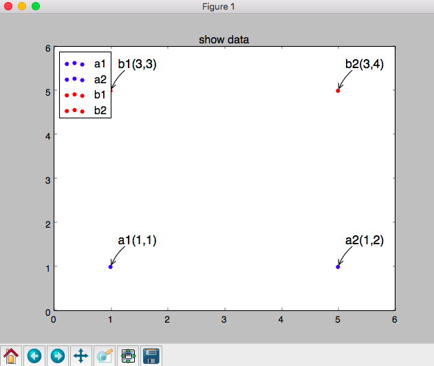
a1、a2表A類,b1、b2表B類,此時入c如下:

要怎麼能辨別c為B類?有興趣者可參考程式碼:
import numpy as np a1 = np.array([1, 1]) a2 = np.array([5, 1]) b1 = np.array([1, 5]) b2 = np.array([5, 5]) b3 = np.array([3, 5]) c = np.array([3, 4]) X1, Y1 = a1 X2, Y2 = a2 X3, Y3 = b1 X4, Y4 = b2 X5, Y5 = b3 X6, Y6 = c plt.title(‘show data’) plt.scatter(X1, Y1, color=”blue”, label=”a1″) plt.scatter(X2, Y2, color=”blue”, label=”a2″) plt.scatter(X3, Y3, color=”red”, label=”b1″) plt.scatter(X4, Y4, color=”red”, label=”b2″) plt.scatter(X5, Y5, color=”red”, label=”b3″) plt.scatter(X6, Y6, color=”red”, label=”c”) plt.legend(loc=’upper left’) plt.annotate(r’a1(1,1)’, xy=(X1, Y1), xycoords=’data’, xytext=(+10, +30), textcoords=’offset points’, fontsize=16, arrowprops=dict(arrowstyle=”->”, connectionstyle=”arc3,rad=.2″)) plt.annotate(r’a2(5,1)’, xy=(X2, Y2), xycoords=’data’, xytext=(+10, +30), textcoords=’offset points’, fontsize=16, arrowprops=dict(arrowstyle=”->”, connectionstyle=”arc3,rad=.2″)) plt.annotate(r’b1(1,5)’, xy=(X3, Y3), xycoords=’data’, xytext=(+10, +30), textcoords=’offset points’, fontsize=16, arrowprops=dict(arrowstyle=”->”, connectionstyle=”arc3,rad=.2″)) plt.annotate(r’b2(5,5)’, xy=(X4, Y4), xycoords=’data’, xytext=(+10, +30), textcoords=’offset points’, fontsize=16, arrowprops=dict(arrowstyle=”->”, connectionstyle=”arc3,rad=.2″)) plt.annotate(r’b3(3,5)’, xy=(X5, Y5), xycoords=’data’, xytext=(+10, +30), textcoords=’offset points’, fontsize=16, arrowprops=dict(arrowstyle=”->”, connectionstyle=”arc3,rad=.2″)) plt.annotate(r’c(3,4)’, xy=(X6, Y6), xycoords=’data’, xytext=(+10, +30), textcoords=’offset points’, fontsize=16, arrowprops=dict(arrowstyle=”->”, connectionstyle=”arc3,rad=.2″)) plt.show()程式碼
KNN例1程式碼如下,設k為3(見式3),為取3點極近xy數組。
import numpy as np import math def Euclidean(vec1, vec2): #Euclidean間距算法 npvec1, npvec2 = np.array(vec1), np.array(vec2) return math.sqrt(((npvec1-npvec2)**2).sum()) def Cosine(vec1, vec2): #Cosine間距算法 npvec1, npvec2 = np.array(vec1), np.array(vec2) return npvec1.dot(npvec2)/(math.sqrt((npvec1**2).sum()) * math.sqrt((npvec2**2).sum())) def create_trainset(): trainset_tf = dict() trainset_tf[u’X1, Y1′] = np.array([1, 1]) trainset_tf[u’X2, Y2′] = np.array([5, 1]) trainset_tf[u’X3, Y3′] = np.array([1, 5]) trainset_tf[u’X4, Y4′] = np.array([5, 5]) trainset_tf[u’X5, Y5′] = np.array([3, 5]) trainset_class = dict() trainset_class[u’X1, Y1′] = ‘A’ trainset_class[u’X2, Y2′] = ‘A’ trainset_class[u’X3, Y3′] = ‘B’ trainset_class[u’X4, Y4′] = ‘B’ trainset_class[u’X5, Y5′] = ‘B’ return trainset_tf, trainset_class def knn_classify(input_tf, trainset_tf, trainset_class, k): xy = np.array([0, 0]) tf_distance = dict() print ‘(1) 各點之遙’ for place in trainset_tf.keys(): tf_distance[place] = Euclidean(trainset_tf.get(place), input_tf) print ‘\tTF(%s) = %f’ % (place, tf_distance.get(place)) class_count = dict() print ‘(2) 得K個鄰為類, k = %d’ % k for i, place in enumerate(sorted(tf_distance, key=tf_distance.get, reverse=False)): current_class = trainset_class.get(place) print ‘\tTF(%s) = %f, class = %s’ % (place, tf_distance.get(place), current_class) class_count[current_class] = class_count.get(current_class, 0) + 1 xy = xy + trainset_tf[place] if (i + 1) >= k: break print ‘(3) K鄰均等之x與y –>’ #式3 finalx=float(xy[0])/k finaly=float(xy[1])/k print ‘\tx = %f’ % finalx, ‘, y = %f’% finaly print ‘(4) K個鄰累計,最高者任其終類’ input_class = ” for i, c in enumerate(sorted(class_count, key=class_count.get, reverse=True)): if i == 0: input_class = c print ‘\t%s類, 現%d次’ % (c, class_count.get(c)) print ‘(5) 結果 = %s’ % input_class input_tf = np.array([3, 4]) trainset_tf, trainset_class = create_trainset() knn_classify(input_tf, trainset_tf, trainset_class, k=3)例1程式碼
結果如下:
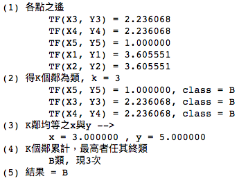
見結果,x於3,y於5。在程式碼中設input_tf = np.array([3, 4]),表x於3,y於4,y於實測與預測相差1,頗為接近!心喜!信心大增!
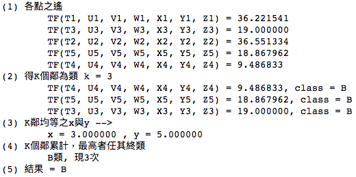
故例2,我設定實測集合於下:
trainset_tf = dict() trainset_tf[u’T1, U1, V1, W1, X1, Y1, Z1′] = np.array([-55, -65, -65, -75, -85, 1, 1]) trainset_tf[u’T2, U2, V2, W2, X2, Y2, Z2′] = np.array([-65, -55, -85, -75, -65, 5, 1]) trainset_tf[u’T3, U3, V3, W3, X3, Y3, Z3′] = np.array([-65, -85, -55, -60, -65, 1, 5]) trainset_tf[u’T4, U4, V4, W4, X4, Y4, Z4′] = np.array([-75, -75, -60, -55, -60, 5, 5]) trainset_tf[u’T5, U5, V5, W5, X5, Y5, Z5′] = np.array([-85, -65, -65, -59, -55, 3, 5]) 以[-55, -65, -65, -75, -85, 1, 1]為例,-55表示手環在第一個接收器的位置,-85離最遠,於空間內置放5個接收器,手環於5個地點發射,故5個接收器的強度都不同。 5個負數代表5個接收器收到的RSSI,後面2個值(1,1)代表xy軸。LinkIt 7697一秒可以送出多筆資料,但這只是模擬數據,實做是要用洗資料的方式,而現在建立的這個資料集是代表實測出來的建模,要給機器去學習比對,找出使用者目前位置。 trainset_class = dict() trainset_class[u’T1, U1, V1, W1, X1, Y1, Z1′] = ‘A’ trainset_class[u’T2, U2, V2, W2, X2, Y2, Z2′] = ‘A’ trainset_class[u’T3, U3, V3, W3, X3, Y3, Z3′] = ‘B’ trainset_class[u’T4, U4, V4, W4, X4, Y4, Z4′] = ‘B’ trainset_class[u’T5, U5, V5, W5, X5, Y5, Z5′] = ‘B’ return trainset_tf, trainset_class 此時,若有人戴手環入室,input_tf代表這人的室內數據。負數為各LinkIt 7697所得RSSI,設xy數分別為零,將由ML算之,設集如下: input_tf = np.array([-72, -72, -63, -53, -63, 0, 0]) ML得x為3, y為5,倒果為因,同上例1之xy得數,由此可看出Machine Learning之強大,何況Deep Learning乎? from matplotlib import pyplot as plt import numpy as np import math def Euclidean(vec1, vec2): #Euclidean間距算法 npvec1, npvec2 = np.array(vec1), np.array(vec2) return math.sqrt(((npvec1-npvec2)**2).sum()) def Cosine(vec1, vec2): #Cosine間距算法 npvec1, npvec2 = np.array(vec1), np.array(vec2) return npvec1.dot(npvec2)/(math.sqrt((npvec1**2).sum()) * math.sqrt((npvec2**2).sum())) def create_trainset(): trainset_tf = dict() trainset_tf[u’T1, U1, V1, W1, X1, Y1, Z1′] = np.array([-55, -65, -65, -75, -85, 1, 1]) trainset_tf[u’T2, U2, V2, W2, X2, Y2, Z2′] = np.array([-65, -55, -85, -75, -65, 5, 1]) trainset_tf[u’T3, U3, V3, W3, X3, Y3, Z3′] = np.array([-65, -85, -55, -60, -65, 1, 5]) trainset_tf[u’T4, U4, V4, W4, X4, Y4, Z4′] = np.array([-75, -75, -60, -55, -60, 5, 5]) trainset_tf[u’T5, U5, V5, W5, X5, Y5, Z5′] = np.array([-85, -65, -65, -59, -55, 3, 5]) trainset_class = dict() trainset_class[u’T1, U1, V1, W1, X1, Y1, Z1′] = ‘A’ trainset_class[u’T2, U2, V2, W2, X2, Y2, Z2′] = ‘A’ trainset_class[u’T3, U3, V3, W3, X3, Y3, Z3′] = ‘B’ trainset_class[u’T4, U4, V4, W4, X4, Y4, Z4′] = ‘B’ trainset_class[u’T5, U5, V5, W5, X5, Y5, Z5′] = ‘B’ return trainset_tf, trainset_class def knn_classify(input_tf, trainset_tf, trainset_class, k): xy = np.array([0, 0]) tf_distance = dict() print ‘(1) 各點之遙’ for place in trainset_tf.keys(): tf_distance[place] = Euclidean(trainset_tf.get(place), input_tf) print ‘\tTF(%s) = %f’ % (place, tf_distance.get(place)) class_count = dict() print ‘(2) 得K個鄰為類 k = %d’ % k for i, place in enumerate(sorted(tf_distance, key=tf_distance.get, reverse=False)): current_class = trainset_class.get(place) print ‘\tTF(%s) = %f, class = %s’ % (place, tf_distance.get(place), current_class) class_count[current_class] = class_count.get(current_class, 0) + 1 xy = [(xy[0] + trainset_tf[place][5]),(xy[1] + trainset_tf[place][6])] if (i + 1) >= k: break print ‘(3) K鄰均等之x與y –>’ finalx=float(xy[0])/k finaly=float(xy[1])/k print ‘\tx = %f’ % finalx, ‘, y = %f’% finaly print ‘(4) K個鄰累計,最高者任其終類’ input_class = ” for i, c in enumerate(sorted(class_count, key=class_count.get, reverse=True)): #擇小排序之 if i == 0: input_class = c print ‘\t%s類, 現%d次’ % (c, class_count.get(c)) print ‘(5) 結果 = %s’ % input_class input_tf = np.array([-72, -72, -63, -53, -63, 0, 0]) trainset_tf, trainset_class = create_trainset() knn_classify(input_tf, trainset_tf, trainset_class, k=3) 結果如下: 此為現實定位模擬數值,接著將有實測之文,ML系列文將以不同風貌展現! (本文同步發表於作者部落格 — 物聯網學習筆記,文章連結;續篇:【Tutorial】運用KNN演算法進行室內定位 Part 2;責任編輯:廖庭儀。) (編按:本文原作為文言文體,風格特殊,有興趣者不妨連回原作拜讀~) 訂閱MakerPRO知識充電報 與40000位開發者一同掌握科技創新的技術資訊!例2實測集合
例2
例2程式碼