Posted By 曾 成訓 on 11 月 21, 2019 in 影像處理, 教學文 | 1 comment

作者：曾成訓（CH.Tseng）

前幾年，我很著迷拍攝一種稱為 Gigapixel panoramas 的相片，就是將數以百張甚至千萬張的相片拼接在一起，成了一張億萬像素的巨幅相片。它的拍攝步驟如下：

1. 找一個寬闊的場景，最好是視野寬達 180 度的壯麗景色。
2. 使用手動或是能自動轉動拍攝的雲台，將高像素且高倍率的相機架上。
3. 由左至右並由上而下，旋轉雲台並確定每個畫面左右上下有 30 % 的重疊。
4. 拍攝完後，在電腦上使用拼接軟體將所有相片接成一張。
5. 將這張高達數十甚至數百 GB 的相片上傳到可支援全景高畫素相片的網站供瀏覽。

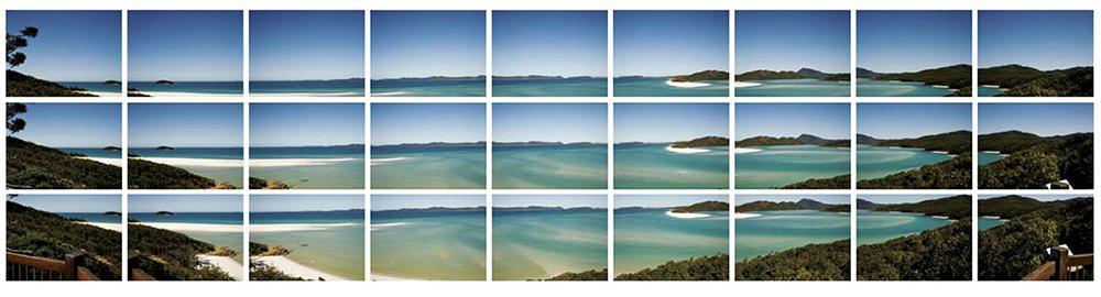
拍攝及拼接方式如下圖所示：

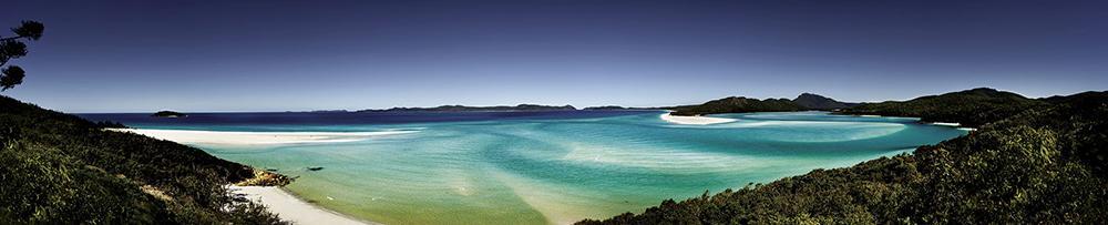
變成：

我所拍攝的巨幅全景

這張是 2011 年 2 月 12 日在三峽鳶山頂拍攝地，總共由 1,863 張相片拼接完成，拼接後的相片總像素為 90 億 pixels。

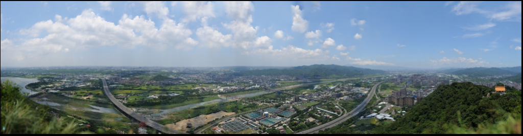
（圖片來源：曾成訓提供）

在這巨幅相片中，可以逐次放大探索細節，下圖是涼亭下正在休息的人：

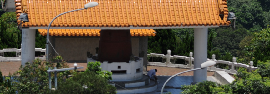
（圖片來源：曾成訓提供）

遠方的軍營：

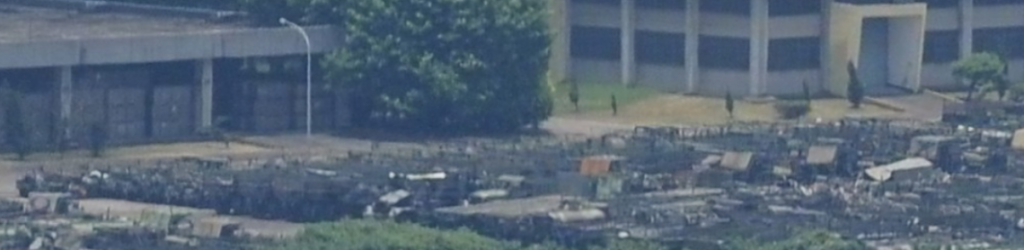
（圖片來源：曾成訓提供）

於象山涼亭拍攝的台北 101，145 億像素：

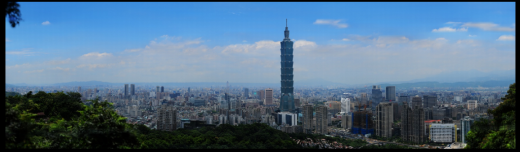
（圖片來源：曾成訓提供）

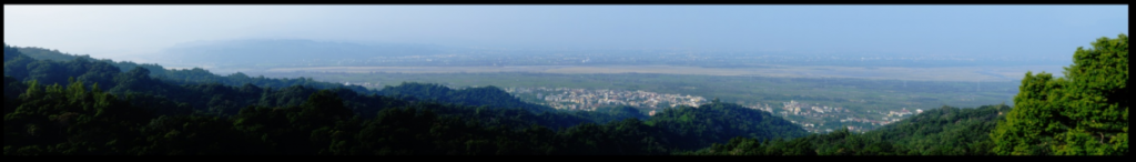
70 億像素的竹東芎林全景，於橫山的大背山山頂拍攝：

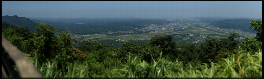
（圖片來源：曾成訓提供）

於樹林大同山遠眺台北盆地，16 億像素：

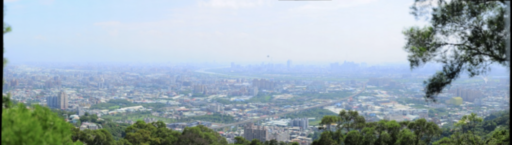
（圖片來源：曾成訓提供）

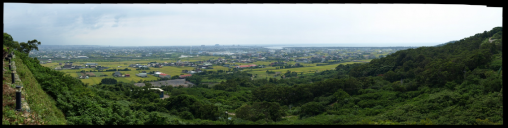
彰化二水鄉全景，於名間鄉的受天官拍攝，約 18 億像素：

（圖片來源：曾成訓提供）

新豐鄕及新竹海岸線，於天德堂前拍攝，約 10 億像素：

（圖片來源：曾成訓提供）

從台北世貿樓上往下拍的兩岸旅展，畫素為 20 億：

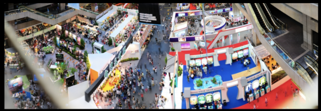
（圖片來源：曾成訓提供）

台中科博館，122 億像素：

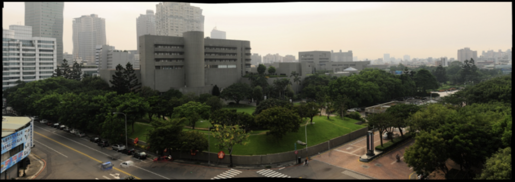
（圖片來源：曾成訓提供）

如何拼接相片

雖然上面介紹了這麼多自己的作品，但這並非重點，重點是瞭解如何用影像處理來拼接全景的相片。最基本的拼接方式是採用所謂的「feature based image alignment」，也就是抓取兩張相片的特徵點，然後將相對應的點對接在一起，其步驟可簡述如下：

1. 找出並篩選相片中的 Keypoints/Descriptors 及對應點，例如：cv2.ORB_create –> cv2.DescriptorMatcher_create
2. 取得 homography matrix，例如：cv2.findHomography
3. 依步驟二產生的 matrix 變形第二張的圖片，例如：cv2.warpPerspective
4. 合併第一張及處理後的第二張圖片即可得到拼接後的結果

特徵點偵測的選擇

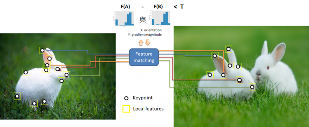
在影像中，容易被視為特徵點的不外乎是 edges、corners、blobs 等，我們將這些具有形狀特性的區域為關鍵點 keypoints，針對這些關鍵點計算並提取該特徵區域的 features，就能用來比對相片（或者辨識物體）。

（圖片來源：曾成訓提供）

其中，Keypoint detection 的演算法有很多種，OpenCV 就提供了超過十一種的方法，像是：

1. FAST – FastFeatureDetector
2. STAR – StarFeatureDetector
3. SIFT – SIFT（nonfree module）
4. SURF – SURF（nonfree module）
5. ORB – ORB
6. BRISK – BRISK
7. MSER – MSER
8. GFTT – GoodFeaturesToTrackDetector
9. HARRIS – GoodFeaturesToTrackDetector with Harris detector enabled
10. Dense – DenseFeatureDetector
11. SimpleBlob – SimpleBlobDetector

還有以下二種方式，可和上述方法合併使用：

• Grid–GridAdaptedFeatureDetector
• Pyramid–PyramidAdaptedFeatureDetector

後方再 append 上述的各個 feature detector name 即可，例如：GridFAST、PyramidSTAR。

在拼接相片時，您可以選用任意的特徵點偵測方法，而下方以 ORB 為例作為相片拼接的示範。ORB 繼承了 FAST 運算快速特性，適用於 realtime，且其針對 FAST 方法進行強化，加入旋轉不變性（rotation invariance）。

1. Pyramid 圖像尺寸並進行各尺寸的 FAST 計算。
2. 使用 Harris keypoint detector 的方法計算每個 keypoint 分數（是否近似 corner？），並進行排序，最多僅取 500 個 keypoints，其餘丟棄。
3. 加入旋轉不變性，使用「intensity centroid」計算每個 keypoint 的 rotation。

程式說明

本程式參考自 School of AI 的課程。

#載入必要模組
from __future__ import print_function
import cv2
import numpy as np

#最多自動取幾個keypoints
MAX_FEATURES = 500
#取得的keypoints都有分數，設定程式僅取最佳的前15%
GOOD_MATCH_PERCENT = 0.15

#進行兩張相片的拼接
def alignImages(im1, im2):
  # 轉為灰階
  im1Gray = cv2.cvtColor(im1, cv2.COLOR_BGR2GRAY)
  im2Gray = cv2.cvtColor(im2, cv2.COLOR_BGR2GRAY)
  
  # 偵測 ORB keypoints及取得descriptors.
  orb = cv2.ORB_create(MAX_FEATURES)
  keypoints1, descriptors1 = orb.detectAndCompute(im1Gray, None)
  keypoints2, descriptors2 = orb.detectAndCompute(im2Gray, None)

  im1Keypoints = np.array([])
　# cv2.drawKeypoints的參數有五個：原始圖片、keypoints、輸出的結果圖片、繪製顏色、繪圖功能設定。
  im1Keypoints = cv2.drawKeypoints(image1, keypoints1, im1Keypoints, color=(0,0,255),flags=0)
  print("Saving Image with Keypoints"); 
  cv2.imwrite("keypoints.jpg", im1Keypoints)

  # 特徵匹配.
  matcher = cv2.DescriptorMatcher_create(cv2.DESCRIPTOR_MATCHER_BRUTEFORCE_HAMMING)
  print(descriptors1, descriptors2)
  matches = matcher.match(descriptors1, descriptors2, None)
  
  # 每個匹配到的特徵帶有分數，由小至大排序
  matches.sort(key=lambda x: x.distance, reverse=False)

  # 僅保留前15%分數較高的匹配特徵
  numGoodMatches = int(len(matches) * GOOD_MATCH_PERCENT)
  matches = matches[:numGoodMatches]

  # 繪出兩張相片匹配的特徵點
  imMatches = cv2.drawMatches(im1, keypoints1, im2, keypoints2, matches, None)
  print("Saving Image with matches"); 
  cv2.imwrite("matches.jpg", imMatches)
  
  # 分別將兩張相片匹配的特徵點匯出
  points1 = np.zeros((len(matches), 2), dtype=np.float32)
  points2 = np.zeros((len(matches), 2), dtype=np.float32)

  for i, match in enumerate(matches):
    points1[i, :] = keypoints1[match.queryIdx].pt
    points2[i, :] = keypoints2[match.trainIdx].pt

  # 找到homography。
  h, mask = cv2.findHomography(points2, points1, cv2.RANSAC)

  # 套用homography
  im1Height, im1Width, channels = im1.shape
  im2Height, im2Width, channels = im2.shape

  im2Aligned = cv2.warpPerspective(im2, h, (im2Width + im1Width, im2Height))

  # 將image1圖像置換到對齊好的圖片中
  stitchedImage = np.copy(im2Aligned)
  stitchedImage[0:im1Height,0:im1Width] = image1
  
  return im2Aligned, stitchedImage

if __name__ == '__main__':
  
  imageFile1 = "my/d1.JPEG"
  print("Reading First image : ", imageFile1)
  image1 = cv2.imread(imageFile1, cv2.IMREAD_COLOR)
  cv2.imshow("First image ",image1)
  cv2.waitKey(0)

  imageFile2 = "my/d2.JPEG"
  print("Reading Second Image : ", imageFile2);  
  image2 = cv2.imread(imageFile2, cv2.IMREAD_COLOR)
  
  print("Aligning images ...")
  im2Aligned, stitchedImage = alignImages(image1, image2)
  print("Saving aligned image"); 
  cv2.imwrite("aligned-image.jpg", im2Aligned)
  cv2.imshow("aligned image ", im2Aligned)

  print("Saving stitched image"); 
  cv2.imwrite("stitched-image.jpg", stitchedImage)
  cv2.imshow("stitched image ", stitchedImage)

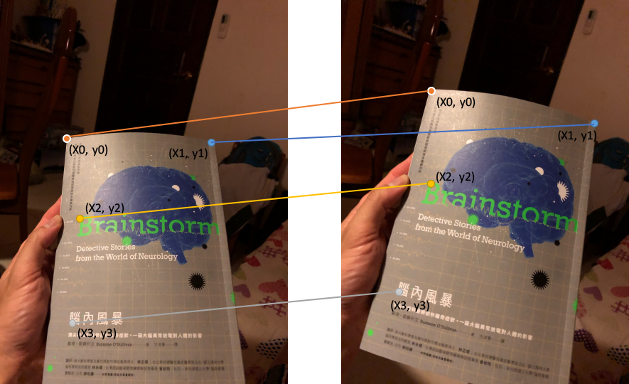
其中比較值得研究的是 cv2.findHomography 這個指令。所謂的 Homography（單應性）字面上很難解釋，但在影像處理的世界裡，一組 3×3 的單應性矩陣（homography matrix），可以讓一個 2D 平面上的所有點，與該矩陣乘積後對應到另一個變形的 2D 平面，而 findHomography 便是找出這個 matrix 的魔術師，只要給它兩組相互對應（順序相同）的 keypoints 就可以。

（圖片來源：曾成訓提供）

因此程式中 cv2.findHomography 所輸出的 h 就是 homography matrix，將它輸入到 cv2.warpPerspective 後，第二張圖片便能依據該 homography matrix 進行變形，變形後的圖片便能與第一張合併。

（圖片來源：曾成訓提供）

（圖片來源：曾成訓提供）

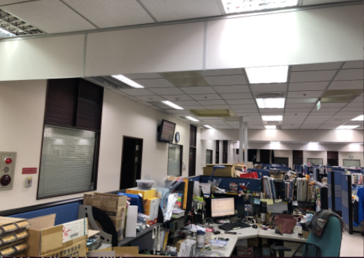
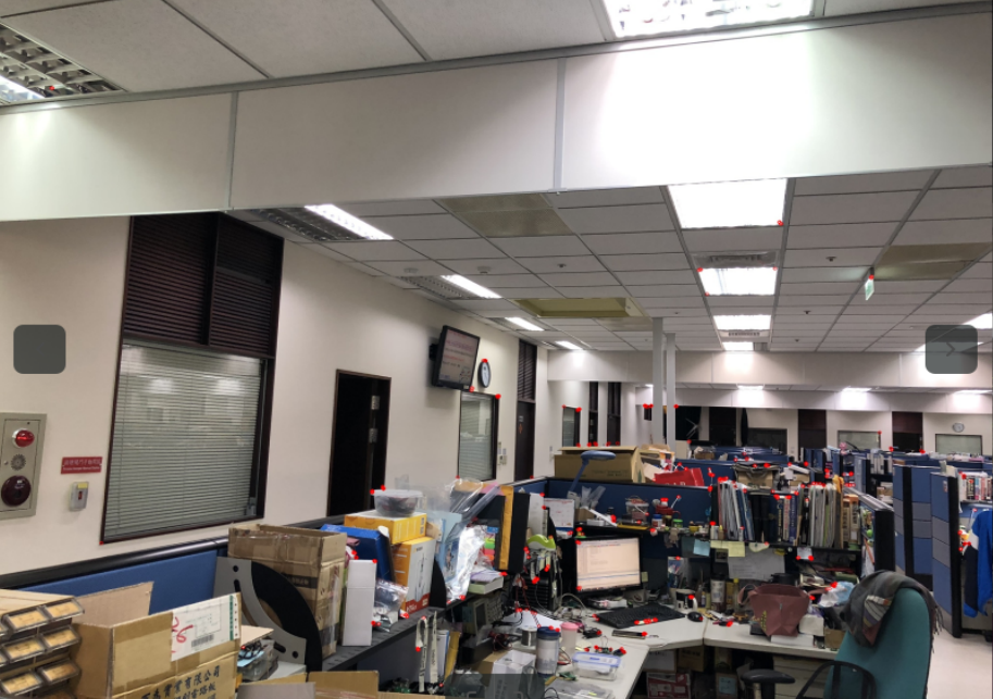
上圖（第一張圖）所抓取的 keypoints（下圖的紅點）：

（圖片來源：曾成訓提供）

keypoints 映射：

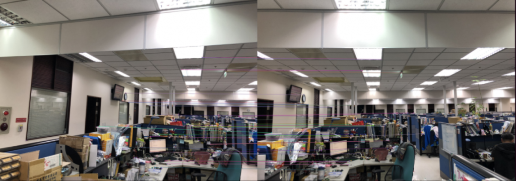
（圖片來源：曾成訓提供）

拼接結果：

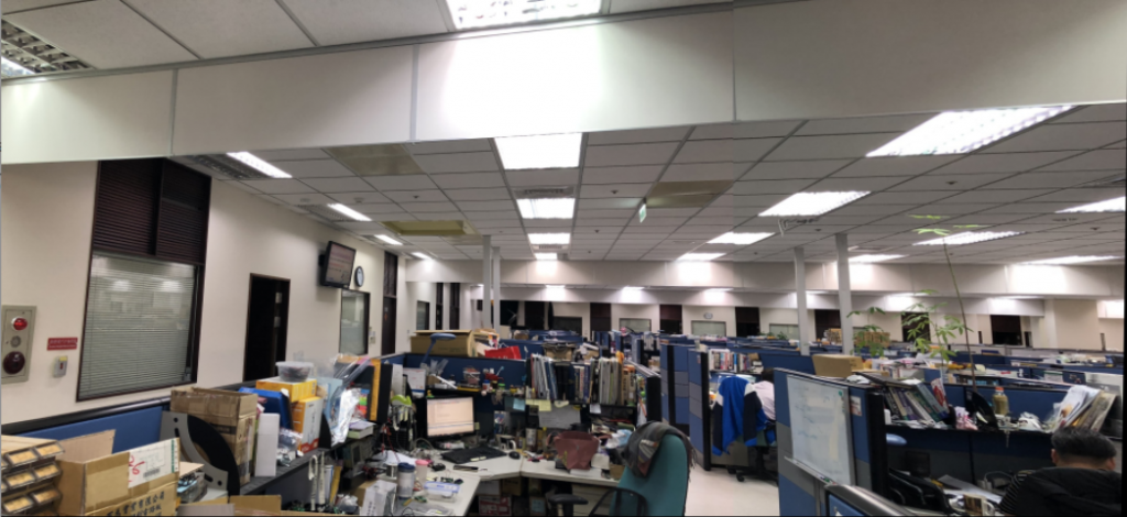
（圖片來源：曾成訓提供）

快速拼接多圖

事實上，OpenCV 內建了一個 Stitcher class 可執行快速的多圖拼接，而且效果相當不錯。使用方式如下，只需要兩行程式，便能得到拼接完成的圖片：

stitcher = cv2.Stitcher.create()
status, result = stitcher.stitch(images)

（注意：舊版本的 OpenCV 使用的是：stitcher = cv2.createStitcher()）

以下面以手機拍攝的 2×4 張相片為例：

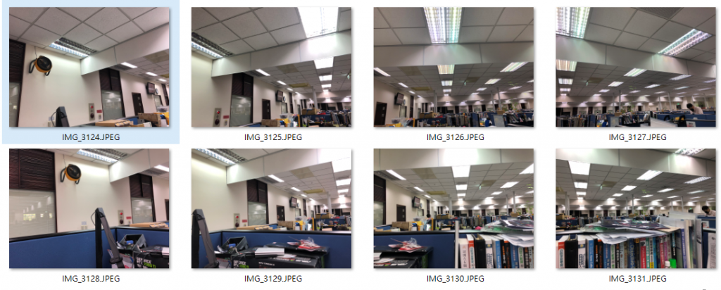
（圖片來源：曾成訓提供）

透過 cv2.Stitcher 的拼接結果：

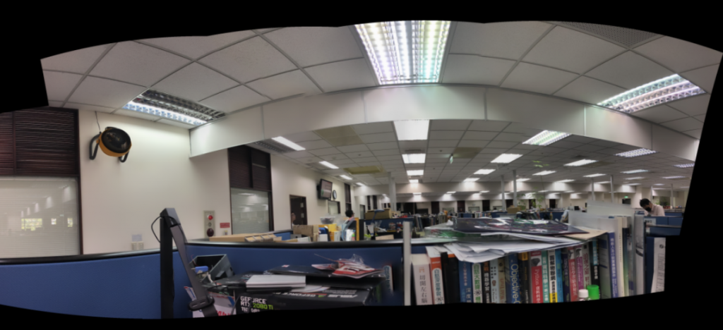
（圖片來源：曾成訓提供）

（本文經作者同意轉載自 CH.TSENG 部落格、原文連結；責任編輯：賴佩萱）

• About
• Latest Posts

曾 成訓

人到中年就像沒對準的描圖紙，一點一點的錯開，我只能當個Maker來使它復位。

Latest posts by 曾 成訓 (see all)

• 【模型訓練】訓練馬賽克消除器 - 2020/04/27
• 【AI模型訓練】真假分不清！訓練假臉產生器 - 2020/04/13
• 【AI防疫DIY】臉部辨識＋口罩偵測＋紅外線測溫 - 2020/03/23